Toggle navigation

.rst .pdf

repository open issue suggest edit

Contents

Tesseroids

When our region of interest covers several longitude and latitude degrees, utilizing Cartesian coordinates to model geological structures might introduce significant errors: they don’t take into account the curvature of the Earth. Instead, we would need to work in Spherical coordinates. A common approach to forward model bodies in geocentric spherical coordinates is to make use of tesseroids.

A tesseroid (a.k.a spherical prism) is a three dimensional body defined by the volume contained by two longitudinal boundaries, two latitudinal boundaries and the surfaces of two concentric spheres of different radii (see Figure: Tesseroid).

Figure: Tesseroid

Tesseroid defined by two longitude coordinates (\(\lambda_1\) and \(\lambda_2\)), two latitude coordinates (\(\phi_1\) and \(\phi_2\)) and the surfaces of two concentric spheres of radii \(r_1\) and \(r_2\). This figure is a modified version of [Uieda2015].

Through the harmonica.tesseroid_gravity function we can calculate the gravitational field of any tesseroid with a given density on any computation point. Each tesseroid can be represented through a tuple containing its six boundaries in the following order: west, east, south, north, bottom, top, where the former four are its longitudinal and latitudinal boundaries in decimal degrees and the latter two are the two radii given in meters.

Note

The harmonica.tesseroid_gravity numerically computed the gravitational fields of tesseroids by applying a method that applies the Gauss-Legendre Quadrature along with a bidimensional adaptive discretization algorithm. Refer to [Soler2019] for more details.

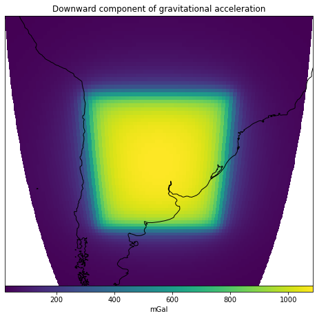
Lets define a single tesseroid and compute the gravitational potential it generates on a regular grid of computation points located at 10 km above its top boundary.

Get the WGS84 reference ellipsoid from boule so we can obtain its mean radius:

import boule as bl

ellipsoid = bl.WGS84
mean_radius = ellipsoid.mean_radius

Define the tesseroid and its density (in kg per cubic meters):

tesseroid = (-70, -50, -40, -20, mean_radius - 10e3, mean_radius)
density = 2670

Define a set of computation points located on a regular grid at 100 km above the top surface of the tesseroid:

import verde as vd

coordinates = vd.grid_coordinates(
    region=[-80, -40, -50, -10],
    shape=(80, 80),
    extra_coords=100e3 + mean_radius,
)

Lets compute the downward component of the gravitational acceleration it generates on the computation point:

import harmonica as hm

gravity = hm.tesseroid_gravity(coordinates, tesseroid, density, field="g_z")

Important

The downward component \(g_z\) of the gravitational acceleration computed in spherical coordinates corresponds to \(-g_r\), where \(g_r\) is the radial component.

And finally plot the computed gravitational field

import matplotlib.pyplot as plt
import cartopy.crs as ccrs

fig = plt.figure(figsize=(8, 9))
ax = plt.axes(projection=ccrs.Orthographic(central_longitude=-60))
img = ax.pcolormesh(
    coordinates[0], coordinates[1], gravity, transform=ccrs.PlateCarree()
)
plt.colorbar(img, ax=ax, pad=0, aspect=50, orientation="horizontal", label="mGal")
ax.coastlines()
ax.set_title("Downward component of gravitational acceleration")
plt.show()

Multiple tesseroids

We can compute the gravitational field of a set of tesseroids by passing a list of them, where each tesseroid is defined as mentioned before, and then making a single call of the harmonica.tesseroid_gravity function.

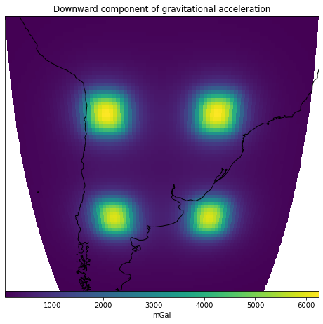
Lets define a set of four prisms along with their densities:

tesseroids = [
    [-70, -65, -40, -35, mean_radius - 100e3, mean_radius],
    [-55, -50, -40, -35, mean_radius - 100e3, mean_radius],
    [-70, -65, -25, -20, mean_radius - 100e3, mean_radius],
    [-55, -50, -25, -20, mean_radius - 100e3, mean_radius],
]
densities = [2670 , 2670, 2670, 2670]

Compute their gravitational effect on a grid of computation points:

coordinates = vd.grid_coordinates(
    region=[-80, -40, -50, -10],
    shape=(80, 80),
    extra_coords=100e3 + mean_radius,
)
gravity = hm.tesseroid_gravity(coordinates, tesseroids, densities, field="g_z")

And plot the results:

fig = plt.figure(figsize=(8, 9))
ax = plt.axes(projection=ccrs.Orthographic(central_longitude=-60))
img = ax.pcolormesh(
    coordinates[0], coordinates[1], gravity, transform=ccrs.PlateCarree()
)
plt.colorbar(img, ax=ax, pad=0, aspect=50, orientation="horizontal", label="mGal")
ax.coastlines()
ax.set_title("Downward component of gravitational acceleration")
plt.show()

Tesseroids with variable density

The harmonica.tesseroid_gravity is capable of computing the gravitational effects of tesseroids whose density is defined through a continuous function of the radial coordinate. This is achieved by the application of the method introduced in [Soler2021].

To do so we need to define a regular Python function for the density, which should have a single argument (the radius coordinate) and return the density of the tesseroids at that radial coordinate. In addition, we need to decorate the density function with numba.jit(nopython=True) or numba.njit for short.

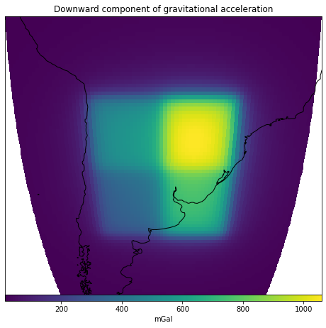
Lets compute the gravitational effect of four tesseroids whose densities are given by a custom linear density function.

Start by defining the tesseroids

tesseroids = (
    [-70, -60, -40, -30, mean_radius - 3e3, mean_radius],
    [-70, -60, -30, -20, mean_radius - 5e3, mean_radius],
    [-60, -50, -40, -30, mean_radius - 7e3, mean_radius],
    [-60, -50, -30, -20, mean_radius - 10e3, mean_radius],
)

Then, define a linear density function. We need to use the jit decorator so Numba can run the forward model efficiently.

from numba import njit

@njit
def density(radius):
    """Linear density function"""
    top = mean_radius
    bottom = mean_radius - 10e3
    density_top = 2670
    density_bottom = 3000
    slope = (density_top - density_bottom) / (top - bottom)
    return slope * (radius - bottom) + density_bottom

Lets create a set of computation points located on a regular grid at 100km above the mean Earth radius:

coordinates = vd.grid_coordinates(
    region=[-80, -40, -50, -10],
    shape=(80, 80),
    extra_coords=100e3 + ellipsoid.mean_radius,
)

And compute the gravitational fields the tesseroids generate:

gravity = hm.tesseroid_gravity(coordinates, tesseroids, density, field="g_z")

Finally, lets plot it:

fig = plt.figure(figsize=(8, 9))
ax = plt.axes(projection=ccrs.Orthographic(central_longitude=-60))
img = ax.pcolormesh(*coordinates[:2], gravity, transform=ccrs.PlateCarree())
plt.colorbar(img, ax=ax, pad=0, aspect=50, orientation="horizontal", label="mGal")
ax.coastlines()
ax.set_title("Downward component of gravitational acceleration")
plt.show()

previous

Rectangular prisms

next

Gravity Disturbance