Tesseroids with variable density
Note
Click here to download the full example code
Tesseroids with variable density
The harmonica.tesseroid_gravity is capable of computing the
gravitational effects of tesseroids whose density is defined through
a continuous function of the radial coordinate. This is achieved by the
application of the method introduced in [Soler2021].
To do so we need to define a regular Python function for the density, which
should have a single argument (the radius coordinate) and return the
density of the tesseroids at that radial coordinate.
In addition, we need to decorate the density function with
numba.jit(nopython=True) or numba.njit for short.
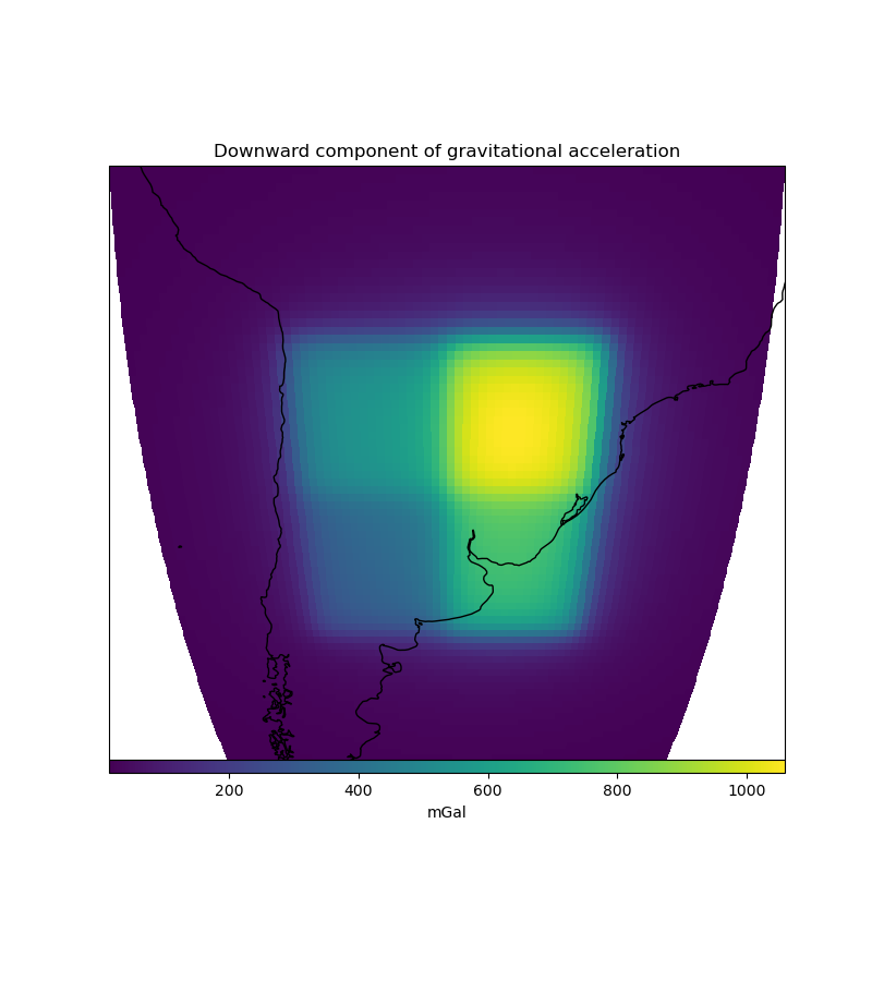
On this example we will show how we can compute the gravitational effect of
four tesseroids whose densities are given by a custom linear density
function.

Out:
[[15.64931026 15.84632554 16.04629019 ... 17.73106017 17.50445005
  17.28024265]
 [15.93321711 16.14345748 16.35722954 ... 18.16928493 17.9230556
  17.68001566]
 [16.2246854  16.4491229  16.6777669  ... 18.62722145 18.3593706
  18.09566506]
 ...
 [15.52398623 15.81724318 16.12003228 ... 18.50055111 18.12075672
  17.75302149]
 [15.24656009 15.52448978 15.8108793  ... 18.06017674 17.705425
  17.36104098]
 [14.97689905 15.24046063 15.51153133 ... 17.6376896  17.30600261
  16.98321625]]
import boule as bl
import cartopy.crs as ccrs
import matplotlib.pyplot as plt
import verde as vd
from numba import njit

import harmonica as hm

# Use the WGS84 ellipsoid to obtain the mean Earth radius which we'll use to
# reference the tesseroid
ellipsoid = bl.WGS84
mean_radius = ellipsoid.mean_radius

# Define tesseroid with top surface at the mean Earth radius, a thickness of
# 10km and a linear density function
tesseroids = (
    [-70, -60, -40, -30, mean_radius - 3e3, mean_radius],
    [-70, -60, -30, -20, mean_radius - 5e3, mean_radius],
    [-60, -50, -40, -30, mean_radius - 7e3, mean_radius],
    [-60, -50, -30, -20, mean_radius - 10e3, mean_radius],
)

# Define a linear density function. We should use the jit decorator so Numba
# can run the forward model efficiently.


@njit
def density(radius):
    """Linear density function"""
    top = mean_radius
    bottom = mean_radius - 10e3
    density_top = 2670
    density_bottom = 3000
    slope = (density_top - density_bottom) / (top - bottom)
    return slope * (radius - bottom) + density_bottom


# Define computation points on a regular grid at 100km above the mean Earth
# radius
coordinates = vd.grid_coordinates(
    region=[-80, -40, -50, -10],
    shape=(80, 80),
    extra_coords=100e3 + ellipsoid.mean_radius,
)

# Compute the radial component of the acceleration
gravity = hm.tesseroid_gravity(coordinates, tesseroids, density, field="g_z")
print(gravity)

# Plot the gravitational field
fig = plt.figure(figsize=(8, 9))
ax = plt.axes(projection=ccrs.Orthographic(central_longitude=-60))
img = ax.pcolormesh(*coordinates[:2], gravity, transform=ccrs.PlateCarree())
plt.colorbar(img, ax=ax, pad=0, aspect=50, orientation="horizontal", label="mGal")
ax.coastlines()
ax.set_title("Downward component of gravitational acceleration")
plt.show()
Total running time of the script: ( 0 minutes 2.865 seconds)
