Upward derivative of a regular grid
Note
Click here to download the full example code
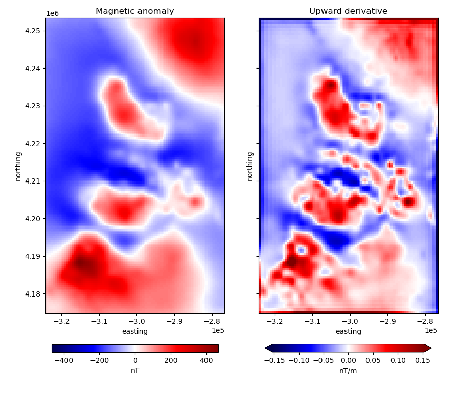
Upward derivative of a regular grid
Out:
Upward derivative:
 <xarray.DataArray (northing: 157, easting: 95)>
array([[ 0.08118127,  0.04840311,  0.04986904, ..., -0.04998174,
        -0.04946451, -0.08324109],
       [ 0.04715736,  0.00822274,  0.00748728, ..., -0.02351687,
        -0.02195097, -0.06526992],
       [ 0.04793475,  0.00739243,  0.00510616, ..., -0.03223078,
        -0.03044794, -0.07926779],
       ...,
       [-0.15958524, -0.04712847, -0.05012313, ...,  0.09228404,
         0.08211778,  0.26426587],
       [-0.14767232, -0.04100584, -0.04493305, ...,  0.08538301,
         0.07280294,  0.24507784],
       [-0.22975479, -0.14307243, -0.15089174, ...,  0.28623612,
         0.25756289,  0.38850882]])
Coordinates:
  * northing  (northing) float64 4.175e+06 4.176e+06 ... 4.253e+06 4.253e+06
  * easting   (easting) float64 -3.24e+05 -3.235e+05 ... -2.774e+05 -2.769e+05
import matplotlib.pyplot as plt
import numpy as np
import pyproj
import verde as vd
import xrft

import harmonica as hm

# Fetch the sample total-field magnetic anomaly data from Great Britain
data = hm.datasets.fetch_britain_magnetic()

# Slice a smaller portion of the survey data to speed-up calculations for this
# example
region = [-5.5, -4.7, 57.8, 58.5]
inside = vd.inside((data.longitude, data.latitude), region)
data = data[inside]

# Since this is a small area, we'll project our data and use Cartesian
# coordinates
projection = pyproj.Proj(proj="merc", lat_ts=data.latitude.mean())
easting, northing = projection(data.longitude.values, data.latitude.values)
coordinates = (easting, northing, data.altitude_m)

# Grid the scatter data using an equivalent layer
eql = hm.EquivalentSources(depth=1000, damping=1).fit(
    coordinates, data.total_field_anomaly_nt
)

grid_coords = vd.grid_coordinates(
    region=vd.get_region(coordinates), spacing=500, extra_coords=1500
)
grid = eql.grid(grid_coords, data_names=["magnetic_anomaly"])
grid = grid.magnetic_anomaly

# Pad the grid to increase accuracy of the FFT filter
pad_width = {
    "easting": grid.easting.size // 3,
    "northing": grid.northing.size // 3,
}
grid = grid.drop_vars("upward")  # drop extra coordinates due to bug in xrft.pad
grid_padded = xrft.pad(grid, pad_width)

# Compute the upward derivative of the grid
deriv_upward = hm.derivative_upward(grid_padded)

# Unpad the derivative grid
deriv_upward = xrft.unpad(deriv_upward, pad_width)

# Show the upward derivative
print("\nUpward derivative:\n", deriv_upward)

# Plot original magnetic anomaly and the upward derivative
fig, (ax1, ax2) = plt.subplots(
    nrows=1, ncols=2, figsize=(9, 8), sharex=True, sharey=True
)

# Plot the magnetic anomaly grid
grid.plot(
    ax=ax1,
    cmap="seismic",
    cbar_kwargs={"label": "nT", "location": "bottom", "shrink": 0.8, "pad": 0.08},
)
ax1.set_title("Magnetic anomaly")

# Plot the upward derivative
scale = np.quantile(np.abs(deriv_upward), q=0.98)  # scale the colorbar
deriv_upward.plot(
    ax=ax2,
    vmin=-scale,
    vmax=scale,
    cmap="seismic",
    cbar_kwargs={"label": "nT/m", "location": "bottom", "shrink": 0.8, "pad": 0.08},
)
ax2.set_title("Upward derivative")

# Scale the axes
for ax in (ax1, ax2):
    ax.set_aspect("equal")

# Set ticklabels with scientific notation
ax1.ticklabel_format(axis="x", style="sci", scilimits=(-2, 2))
ax1.ticklabel_format(axis="y", style="sci", scilimits=(-2, 2))

plt.tight_layout()
plt.show()
Total running time of the script: ( 0 minutes 10.893 seconds)