Note
Go to the end to download the full example code
Tesseroids with variable density#
The harmonica.tesseroid_gravity is capable of computing the
gravitational effects of tesseroids whose density is defined through
a continuous function of the radial coordinate. This is achieved by the
application of the method introduced in [Soler2021].
To do so we need to define a regular Python function for the density, which
should have a single argument (the radius coordinate) and return the
density of the tesseroids at that radial coordinate.
In addition, we need to decorate the density function with
numba.jit(nopython=True) or numba.njit for short.
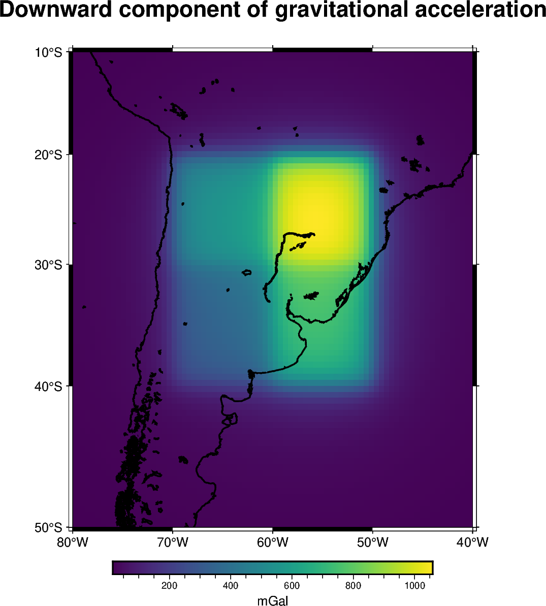
On this example we will show how we can compute the gravitational effect of
four tesseroids whose densities are given by a custom linear density
function.

[[15.65235898 15.84941264 16.04941625 ... 17.73451444 17.50786018
  17.2836091 ]
 [15.93632114 16.14660247 16.36041617 ... 18.17282458 17.92654728
  17.68345999]
 [16.22784621 16.45232743 16.68101597 ... 18.63085032 18.36294728
  18.09919036]
 ...
 [15.52701053 15.82032461 16.1231727  ... 18.50415529 18.12428691
  17.75648004]
 [15.24953035 15.52751418 15.81395949 ... 18.06369513 17.70887428
  17.36442317]
 [14.97981677 15.2434297  15.51455321 ... 17.64112568 17.30937408
  16.98652484]]
import boule as bl
import pygmt
import verde as vd
from numba import njit

import harmonica as hm

# Use the WGS84 ellipsoid to obtain the mean Earth radius which we'll use to
# reference the tesseroid
ellipsoid = bl.WGS84
mean_radius = ellipsoid.mean_radius

# Define tesseroid with top surface at the mean Earth radius, a thickness of
# 10km and a linear density function
tesseroids = (
    [-70, -60, -40, -30, mean_radius - 3e3, mean_radius],
    [-70, -60, -30, -20, mean_radius - 5e3, mean_radius],
    [-60, -50, -40, -30, mean_radius - 7e3, mean_radius],
    [-60, -50, -30, -20, mean_radius - 10e3, mean_radius],
)

# Define a linear density function. We should use the jit decorator so Numba
# can run the forward model efficiently.


@njit
def density(radius):
    """Linear density function"""
    top = mean_radius
    bottom = mean_radius - 10e3
    density_top = 2670
    density_bottom = 3000
    slope = (density_top - density_bottom) / (top - bottom)
    return slope * (radius - bottom) + density_bottom


# Define computation points on a regular grid at 100km above the mean Earth
# radius
coordinates = vd.grid_coordinates(
    region=[-80, -40, -50, -10],
    shape=(80, 80),
    extra_coords=100e3 + ellipsoid.mean_radius,
)

# Compute the radial component of the acceleration
gravity = hm.tesseroid_gravity(coordinates, tesseroids, density, field="g_z")
print(gravity)
grid = vd.make_xarray_grid(
    coordinates, gravity, data_names="gravity", extra_coords_names="extra"
)

# Plot the gravitational field
fig = pygmt.Figure()

title = "Downward component of gravitational acceleration"

with pygmt.config(FONT_TITLE="16p"):
    fig.grdimage(
        region=[-80, -40, -50, -10],
        projection="M-60/-30/10c",
        grid=grid.gravity,
        frame=["a", f"+t{title}"],
        cmap="viridis",
    )

fig.colorbar(cmap=True, frame=["a200f50", "x+lmGal"])

fig.coast(shorelines="1p,black")

fig.show()
Total running time of the script: (0 minutes 3.408 seconds)