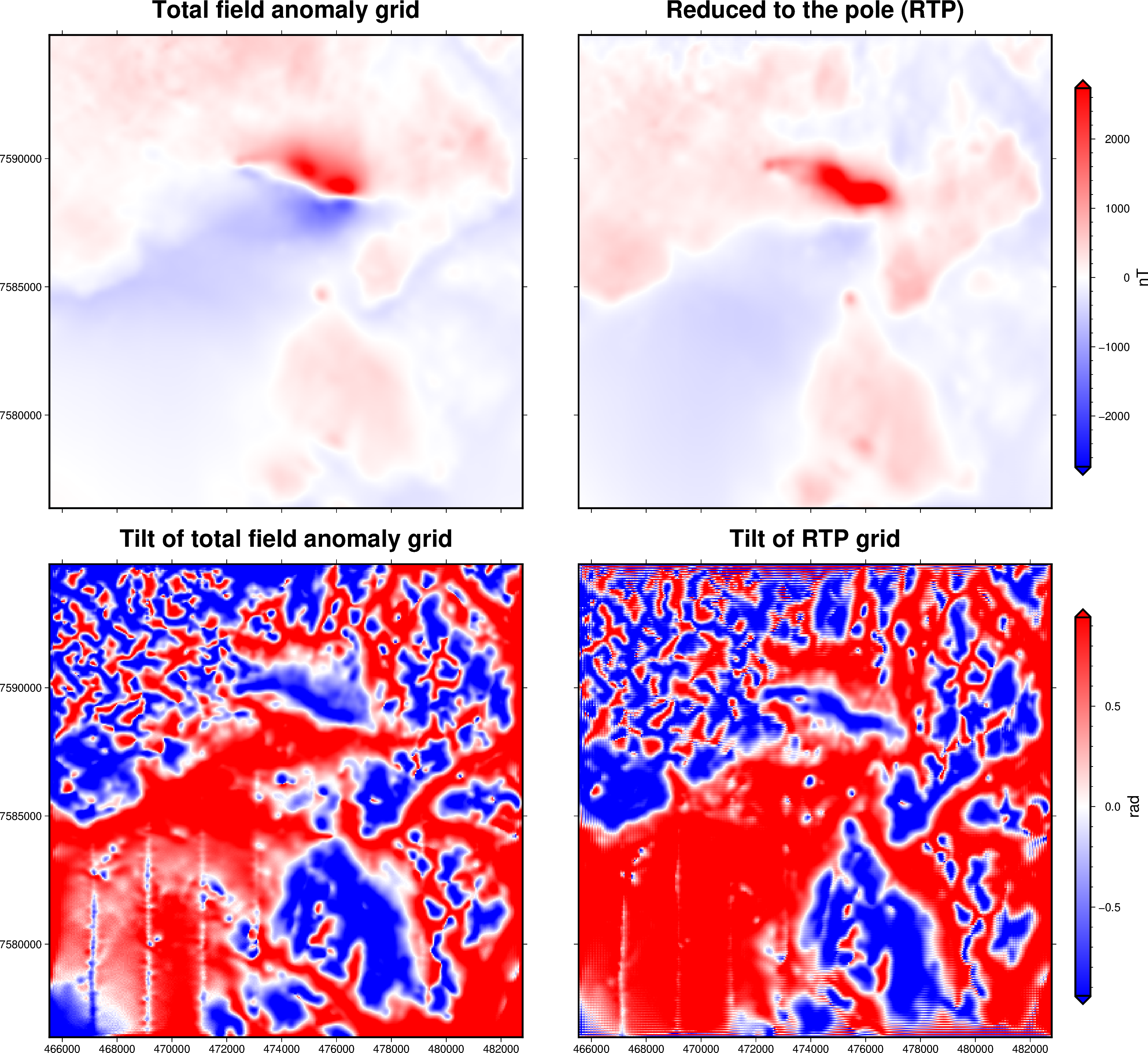
Tilt of a regular grid

Tilt:
 <xarray.DataArray (northing: 370, easting: 346)> Size: 1MB
array([[-1.0783784 , -1.02860717, -1.04340939, ...,  1.03827901,
         1.02638371,  1.08973867],
       [-1.03642874, -1.45715868, -1.48696672, ...,  1.51656355,
         1.5129112 ,  1.02828324],
       [-1.04841707, -1.50371841, -1.54700707, ...,  1.51704351,
         1.51441199,  1.04159331],
       ...,
       [-1.10088333, -1.33804824, -1.31496059, ...,  0.32157698,
         0.72592929,  1.35945242],
       [-1.08740577, -1.34292621, -1.3185706 , ...,  0.24911404,
         0.65291946,  1.37433697],
       [-1.11194247, -1.03333203, -1.04572183, ..., -0.19281687,
         0.64110985,  1.23484722]])
Coordinates:
  * easting   (easting) float64 3kB 4.655e+05 4.656e+05 ... 4.827e+05 4.828e+05
  * northing  (northing) float64 3kB 7.576e+06 7.576e+06 ... 7.595e+06 7.595e+06

Tilt from RTP:
 <xarray.DataArray (northing: 370, easting: 346)> Size: 1MB
array([[-1.21333209, -1.4644687 , -1.46563213, ...,  1.42901118,
         1.38962685,  1.02899332],
       [-1.03471553,  0.11466866, -0.25452967, ..., -0.32908127,
         0.13113278,  0.67459503],
       [-1.17050374, -1.17608165, -1.29967283, ...,  1.33473239,
         1.29156435,  0.91346865],
       ...,
       [-1.2096313 ,  0.31156962, -0.17243796, ...,  0.59752655,
         0.97812607,  1.20524396],
       [-1.21908118, -0.54733936, -0.90922684, ...,  0.17107842,
         0.80343702,  1.21308321],
       [-0.4247845 ,  0.72898686,  0.59961164, ...,  1.04173936,
        -0.14524941,  0.66491492]])
Coordinates:
  * easting   (easting) float64 3kB 4.655e+05 4.656e+05 ... 4.827e+05 4.828e+05
  * northing  (northing) float64 3kB 7.576e+06 7.576e+06 ... 7.595e+06 7.595e+06

import ensaio
import pygmt
import verde as vd
import xarray as xr
import xrft

import harmonica as hm

# Fetch magnetic grid over the Lightning Creek Sill Complex, Australia using
# Ensaio and load it with Xarray
fname = ensaio.fetch_lightning_creek_magnetic(version=1)
magnetic_grid = xr.load_dataarray(fname)

# Pad the grid to increase accuracy of the FFT filter
pad_width = {
    "easting": magnetic_grid.easting.size // 3,
    "northing": magnetic_grid.northing.size // 3,
}
# drop the extra height coordinate
magnetic_grid_no_height = magnetic_grid.drop_vars("height")
magnetic_grid_padded = xrft.pad(magnetic_grid_no_height, pad_width)

# Compute the tilt of the grid
tilt_grid = hm.tilt_angle(magnetic_grid_padded)

# Unpad the tilt grid
tilt_grid = xrft.unpad(tilt_grid, pad_width)

# Show the tilt
print("\nTilt:\n", tilt_grid)

# Define the inclination and declination of the region by the time of the data
# acquisition (1990).
inclination, declination = -52.98, 6.51

# Apply a reduction to the pole over the magnetic anomaly grid. We will assume
# that the sources share the same inclination and declination as the
# geomagnetic field.
rtp_grid_padded = hm.reduction_to_pole(
    magnetic_grid_padded, inclination=inclination, declination=declination
)

# Unpad the reduced to the pole grid
rtp_grid = xrft.unpad(rtp_grid_padded, pad_width)

# Compute the tilt of the padded rtp grid
tilt_rtp_grid = hm.tilt_angle(rtp_grid_padded)

# Unpad the tilt grid
tilt_rtp_grid = xrft.unpad(tilt_rtp_grid, pad_width)

# Show the tilt from RTP
print("\nTilt from RTP:\n", tilt_rtp_grid)

# Plot original magnetic anomaly, its RTP, and the tilt of both
region = (
    magnetic_grid.easting.values.min(),
    magnetic_grid.easting.values.max(),
    magnetic_grid.northing.values.min(),
    magnetic_grid.northing.values.max(),
)
fig = pygmt.Figure()
with fig.subplot(
    nrows=2,
    ncols=2,
    subsize=("20c", "20c"),
    sharex="b",
    sharey="l",
    margins=["1c", "1c"],
):
    scale = 0.5 * vd.maxabs(magnetic_grid, rtp_grid)
    with fig.set_panel(panel=0):
        # Make colormap of data
        pygmt.makecpt(cmap="polar+h", series=[-scale, scale], background=True)
        # Plot magnetic anomaly grid
        fig.grdimage(
            grid=magnetic_grid,
            projection="X?",
            cmap=True,
            frame=["a", "+tTotal field anomaly grid"],
        )
    with fig.set_panel(panel=1):
        # Make colormap of data
        pygmt.makecpt(cmap="polar+h", series=[-scale, scale], background=True)
        # Plot reduced to the pole magnetic anomaly grid
        fig.grdimage(
            grid=rtp_grid,
            projection="X?",
            cmap=True,
            frame=["a", "+tReduced to the pole (RTP)"],
        )
        # Add colorbar
        label = "nT"
        fig.colorbar(
            frame=f"af+l{label}",
            position="JMR+o1/-0.25c+e",
        )

    scale = 0.6 * vd.maxabs(tilt_grid, tilt_rtp_grid)
    with fig.set_panel(panel=2):
        # Make colormap for tilt (saturate it a little bit)
        pygmt.makecpt(cmap="polar+h", series=[-scale, scale], background=True)
        # Plot tilt
        fig.grdimage(
            grid=tilt_grid,
            projection="X?",
            cmap=True,
            frame=["a", "+tTilt of total field anomaly grid"],
        )
    with fig.set_panel(panel=3):
        # Make colormap for tilt rtp (saturate it a little bit)
        pygmt.makecpt(cmap="polar+h", series=[-scale, scale], background=True)
        # Plot tilt
        fig.grdimage(
            grid=tilt_rtp_grid,
            projection="X?",
            cmap=True,
            frame=["a", "+tTilt of RTP grid"],
        )
        # Add colorbar
        label = "rad"
        fig.colorbar(
            frame=f"af+l{label}",
            position="JMR+o1/-0.25c+e",
        )
fig.show()